Field Activity 5: Geodatabases, Attributes and Domains

Introduction

Our task in this field activity was to create a geodatabase in ArcCatalog which we would use in the coming weeks to collect data and ultimately create a microclimate map. Developing and creating a geodatabase may sound like a simple task however it is of great importance to make it correctly. Using ArcCatalog makes the process of creating a geodatabase easy but setting it up properly for data collection is a whole other task in and of itself. In this exercise we worked on pre-planning for a future field activity where we would be using our geodatabase in the field for data collection. This report is divided into two parts: part one focuses on the importance of having the properly set up geodatabase and part two will act as a tutorial on how to the microclimate geodatabase was actually created. 

Methods

Part 1:

It is crucial when conducting field work to be well prepared. In order to properly utilize tools like ArcPad we can install a geodatabase to collect data. Geodatabases can be used to manage and store data when using ArcGIS. Data can then be easily accessed and is a way to organize GIS data. When working toward planning for field work by creating a geodatabase the biggest aspect to consider is the domain. A domain is a range or group of valid attribute values that can be used in order to record features collected in the field. These geodatabases are important because they can ensure that the entry of the data is accurate and also consistent. Single domains can be used for many feature classes within a single geodatabase since the domain is merely a property of the greater geodatabase which can be set. 

There are a number of different domain field types which can be set including: short and long integer, float, double, text and date. These can be used to better classify the data values in order to maintain consistency of the data while in the field. An example of this can be found in our future project. Say that someone wishes to collect land cover type at various points in their study area. The would set their domain as text with predefined values such as snow, grass, gravel, concrete and other. By setting the possible values of the domain it will not only speed up the process of data entry in the field but also serve as a way to standardize data and minimize possible error. It is also important to set ranges for data like temperature to prevent any accidental errors like inputting 200 degrees fahrenheit when you meant to put 20. Setting a reasonable range of 0 to 100 degrees it will help to avoid numerical errors as well. By completing all of this work prior to field work it will save time and frustration of needing to correct for errors later.


Part 2

The process of creating the microclimate map which we will be developing in the coming weeks involves various stages which can be seen below. 

Geodatabase Pre-Planning

It's important when creating a geodatabase to take into consideration before you start making it what the purpose of it is. For instance, in this lab we are working to create a geodatabase to organize microclimate data. Microclimate is basically the climate of a small area that is different than other parts of the surrounding environment. An example of this could be that an area blocked by wind such as the courtyard in Phillips hall or behind another building on campus might be warmer than open areas like the campus mall not that much further away. Microclimates don't have to be limited to a small size though, they can also be large like the comparison of climate in a downtown, urban area compared to a surrounding rural land. 

It's important to determine what information we will need to collect for this map which will ultimately act as a way to visualize microclimates to the viewer. Some data that would be valuable to this study includes: temperature (both at the surface and at eye level), dew point, wind chill, ground cover, wind speed, direction of wind etc. All of these need to be included in plans for our geodatabase for this map.

Creating the Geodatabase

The next step is to actually create the geodatabase itself. The best way to do this is to start by opening ArcCatalog. Then choose a folder in which you want your geodatabase to be created in and right click on the screen and select the option "new" and "file geodatabase" (Fig. 1).

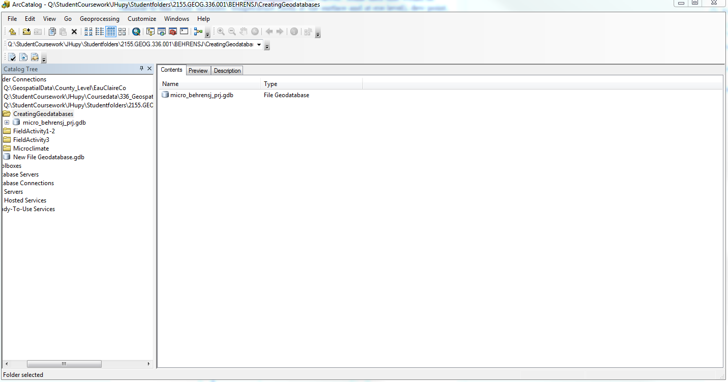
(Fig. 1) This file geodatabase was created and named "micro_behrensj.gdb" since it will be where all the collected microclimate data from the field will be stored until it is analyzed and incorporated into the final microclimate map.

Setting Up Geodatabase Domains

Creating the domains in a geodatabase is very important to do correctly but can often be the most tricky part of geodatabase set up. Domains can be defined as rules that are applied to a field within a table which work to enforce the integrity of data by making it so that only the predetermined values for specific domains can entered. In this case to set the domains you right click on the geodatabase that you created and select the "properties" option. Then by selecting the "domains" tab you can set the domains and their ranges (Fig. 2).

(Fig. 2) Within the domains tab there are tables where the domain name, description, and other properties can be entered. There can be multiple different domains with different properties within the same geodatabase. This makes it so that you don't need to create as many feature classes but rather can organize your data within the geodatabase itself while collecting the data in the field.

Setting the range values and the field type are the two most challenging decisions that need to be made when assigning domain properties. As can be seen in Fig. 3, all the variables of microclimate which we want to collect data on are listed under the domain name. For example, setting the range for temperature it seems logical to set the minimum value at -30 and the maximum value at 60. Since we will be collecting whole numbers the short integer field type was selected. All of these parameters can be set individually based each domain's different requirements. After all of these steps have been completed you have a well thought out geodatabase that can be used in the field for data collection.

(Fig. 3) The range and field type of the domains are set separately for each of the domains to ensure that they are the best properties fit for the given data that will be collected in each domain.

Conclusion

While I previously had always thought that creating a geodatabase was a simple and rather trivial task I learned through this activity that it can be very important and help to ensure more success in the field. Pre-planning a project using domains to organize data in geodatabases can minimize errors and speed up the process of actually collecting the data values while in the field. Domains are extremely useful in that they minimize the number of feature classes that are created because they can organize data in a way that does not require more than a single class. The creating of a geodatabase prior to field work is crucial and a rather simple way to stay organized.

Field Activity 4: UAS Mission Planning

Introduction

This week's activity was less of a field exercise and more of a research project. We were tasked with conducting research on our own to gain a better understanding of unmanned aerial systems (UAS). In addition to utilizing the software, Real Flight 7.5 to test fly various platforms we were also challenged with addressing real world scenarios which would utilize different UAS technologies. This activity allowed us to get hands on experience using UAS in the flight simulator while also conducting research to better understand how this technology can be used in the field. In addressing the various scenarios we were tasked with determining the best type of UAS platform and other materials that should be used which would be most fit for the project at hand. Throughout this activity we were able to not only expand our knowledge of UAS but also apply this knowledge to address real world situations. 

Overview of UAS

Unmanned aerial systems utilize unmanned aerial vehicles (UAVs) which are aircrafts that have the ability to fly autonomously, or without pilot control. Most UAVs which are amateur are neither military nor commercial and are typically able to fly under the "recreational" exception to the FAA regulations. A common misconception is that these amateur air crafts are able to be flied anywhere by anyone, however the FAA regulates that the UAVs have pilots and programmers within the area to monitor the altitude and distance in which the UAV flies in order to stay within the FAA limits. To operate these crafts, most of the time they are manually flown using remote control to take off and land but when in the air GPS-guided flight plans are utilized to allow the UAV to operate autonomously once at a safe altitude. While they can be in autopilot and navigated based on predetermined flight paths, they are still capable of being flown manually and often are flown this way. Software which equips the UAV with the autopilot capability can either come with the UAV itself or be purchased separately. There is also other software which can be used in mission planning which is quite essential for the use of the aircraft in order to pre-program a certain flight path. As the UAV is flying programmers and pilots are able to remotely analyze the data in real time using various types of graphical interfaces.

Common Types of UAS

Fixed Wing Aircraft

Fixed wing air crafts are basically small planes which are unmanned. Some major benefits to this type of UAV is that they can fly for long periods of time based on how they are powered, they can carry greater payloads than most rotary crafts and they can usually and can more efficiently utilize the power it is given. These types of crafts can be powered by both batteries and gas which can allow for 1-10 hrs of flight time. Since they are able to glide if there is a loss of power they are much more forgiving in the case that there is some type of problem while it is in flight. Some downfalls of this particular UAV include the fact that they require an area that can act as a runway in order to take off and they can vary greatly in price.

(Fig. 1) This is an example of a fixed wing UAV. This is the APM Plane which can be found at the following link: ArduPlane.

Helicopters

Another type of UAV is a helicopter which are single rotary aircrafts. This means that they have a single motor which lifts the craft with 2 or  more blades. A major benefit to this type of craft is that they are capable of vertical takeoffs and can hover to capture more detailed images from below. Hovering also allows for more real-time feedback  which can be analyzed by the pilots and others who are present at the flight. Like the fixed-wing UAVs they can be powered by either gas or electric however their flight time is heavily influenced by the amount of weight they are carrying. This particular type of UAV is very versatile and can carry various weights of equipment, reach high speeds and achieve long flight times depending on the model.

(Fig. 2) This is an example of a helicopter UAV. More information about this particular model can be found using the following link: UAS Vision.

Multicopters

Multicopters are very similar to helicopters however they utilize 4 or more completely separate motors to provide the lift for the craft. There is a great deal of variety in the different types of multicopters which include those with anywhere from 4 to 8 motors that can have greater payloads and increase the overall stability in flight. Due to the increase in the number of motors compared to the helicopter they are able to stay extremely stable even in very strong winds but they do require an on-board computer system in order to fly. Since they have so many motors however, they do not typically have very long flight times but they are able to take very detailed images based on their very stable hovering capabilities. The most common type of multicopter is the quadcopter which has only 4 motors, is the most user friendly and the least complicated. 

(Fig. 3) This is an example of a quadcopter, which is a type of multicopter which utilizes a total of 4 different motors. More information about this particular model can be found using the following link: Robot Shop.

Methods

Flight Simulator

In this portion of the activity we had the opportunity to get some hands on experience with various types of UAVs without actually flying them. Using the Real Flight 7.5 we were able to practice our flying in different environments and with different platforms or aircrafts. I decided to use a helicopter, fixed wing UAV and some other crafts to test out my ability to fly. It was also very interesting to adjust the wind speed as well as change the flight environment. Within this software we were also able to adjust the camera angles from which we viewed the plane we were flying which was an another interesting variable. I really enjoyed the opportunity to work with this software because it gave me a lot of insight that I was able to apply to the various scenarios below since I now had a better understanding of how the different types of UAVs operate. 

Flight Log

Within my flight log I kept track of various elements of all my flights which included: flight number, craft type, environment I was flying in, wind speed in mph, view I was using to fly the aircraft, the amount of flight time I had, if I crashed or not and if so the reason for the crash. All of this data was very important to organize properly so I can better understand how my flying is and what I need more practice on. As can be seen in Fig. 4 I require much more flight time to be logged before I fly an actual UAV.

(Fig. 4) My flight log from using the flight simulator, Real Flight 7.5 which tracked my aircraft type, location, wind speed, flight time and any crashes I had including the reason for the crash.

Scenarios

Scenario 1:
A pineapple plantation has about 8000 acres and they want you to give them an idea of where they have vegetation that is not healthy, as well as help them out with when might be a good time to harvest.

The first thing to address in this scenario is how to determine whether or not the pineapples are healthy or not. Once this has been addressed it can be decided how these techniques can be applied to and utilized with a UAV. Based on background knowledge of remote sensing it is clear that the NIR (near infrared) band of the electromagnetic spectrum is the best way to monitor vegetation health. This is because it has a longer wavelength than visible light. The reflectance in this particular band is so useful in tracking vegetation health because plants are a strong reflector of light of the NIR wavelength. This means that when the NIR wavelength of light hits the plant most of it is reflected off the plant rather than being absorbed. The interaction between the plant cells and the NIR light cause this greater amount of reflection. Based on the amount of reflected light it can be determined that plants that are healthy will reflect more of the NIR light while plants that have damaged cells and are therefore unhealthy allow more NIR light to be absorbed into the plant and therefore not be reflected. 

By utilizing a NIR camera the plants which appear bright are those which are healthy while unhealthy vegetation will have the opposite appearance. Monitoring the amount of reflected light in the NIR wavelength we will be able to track the health of the pineapple plants in the plantation. To apply this idea with looking more closely at how to determine when the pineapples are ready to be harvested or not the NIR camera can also be used. Pineapples that are ready to be harvested will appear at least 1/3 yellow in color. By looking at the reflectance data it would be fairly simple to look at the areas where there is a greater amount of yellow light being reflected to decide if the plants in that area should be harvested. 

UAS are a great way to collect the data which was discussed above. When deciding which particular type of UAV would be best suited for this particular scenario we must think about a few key factors: how large is the area and how long will it need to be in flight. I would not recommend the use of a fixed-wing aircraft because there is not a good area where a fixed-wing aircraft could take off. Since very precise images are need in order to properly analyze the NIR reflectance values I think that a quadcopter with an infrared camera mounted on the bottom of it would be the best option to capture the necessary data. A quadcopter has much more stability and based on the shape it is easy to mount a camera to the bottom of it so we can gain images of the land directly below where the UAV flies. I believe this to be a better option than using a helicopter because they are much more stable and able to support much greater payloads like that of the infrared camera. 

Scenario 2:
A military testing range is having problems engaging in conducting its training exercises due to the presence of desert tortoises. They currently spend millions of dollars doing ground based surveys to find their burrows. They want to know if you, as the geographer can find a better solution with UAS.

Desert tortoises can be found in the deserts in the western United States and area able to survive in quite extreme habitats that other species would have trouble living in. Since it has been found that desert tortoises spent up to 95% of their lives inside their burrows it is of great importance, especially in this scenario, to locate such burrows. Construction of these underground homes for the tortoises requires a special type of soil which is a mixture of gravel and clay rather than sand which can collapse too easily. Biologists have also found that they prefer to construct their burrows around shrub vegetation.

In order to locate these burrows it would be necessary to employ a fixed-wing aircraft which could quickly analyze a very large area. It would be most beneficial to also have a UAV that is gas powered rather than battery powered so that the flight time can be increased since the area of study is so large. The best way to locate these burrows would be to focus on areas where there are shrubs since 97% of the burrows are found near this type of vegetation however it is also important to determine the soil type in the area and the depth of the soil to more accurately locate these desert tortoise homes. In order to do so I would recommend attaching a multi-spectral scanner to the fixed-wing aircraft. Using the thermal band of the electromagnetic spectrum we could gain a better idea of where the tortoises are actually located beneath the surface. It would be important however to collect data at dusk when the ground is cold so that the body heat of the tortoises can better be pin pointed without the heat of the ground disrupting the accuracy of the collected data. 


By analyzing the data collected by the multi-spectral scanner mounted to the fixed-wing UAV we could determine the most appealing areas for the desert tortoises to create a burrow. Then by combining this data with that of thermal data collected we could determine the ideal habitats for the burrows and where the individual tortoises are actually located. We could even further look at the soil nutrients and soil types to determine the best areas where the tortoises would want to dig their burrows. This location information could then be relayed to ground crew teams who would then not need to search nearly as large of an area to find the tortoise burrows and therefore less money would need to be spent on their labor.

Discussion

There is a great deal of variation in the types of UAVs but it is clear that they can be used for a wide variety of real world situations. For the first scenario we were tasked with how to monitor the health of a large plantation of pineapples. I determined that in this particular situation a multicopter, particularly a quadcopter UAV would be best when using NIR imagery in order to determine how healthy the pineapples are. Using this NIR information it would also be possible to track the growth of the plants and decide when it is time for the fruits to be harvested.  In the second scenario,  I was tasked with determining how to locate desert tortoise burrows in a large area. I decided that since it was such a large area to survey that a fixed wing aircraft would be best, especially if it were gas powered which would allow it to cover more area in a single flight. Also, the fixed wing aircraft would need to be fitted with something to detect the visible near infrared band of the electromagnetic spectrum which would allow for greater analysis of the soil types in order to locate the burrow locations. 

In these practice scenarios it was very important to use my previous knowledge of remote sensing techniques, geospatial analysis tools and the information I gained of UAV systems throughout this activity. The scenario exercise was a great way to really challenge my ability to think critically and remind me how important it is to really think about all aspects of the situation and apply all my knowledge toward solving the problem at hand. 

Conclusion

While this activity might not have utilized traditional field work to gain a better understanding of unmanned aerial systems I found this lab very informative. The research portion of this activity required a great deal of research to be conducted and allowed us to gain a better understanding of just how much variety there is in the world of UAVs. Each scenario offered a very realistic situations which we were able to apply all that we learned to it and determine how we would create a proposal for a future employer. I also found it extremely useful to use the flight simulator to gain a better understanding of the benefits and negative features of the different types of UAVs. 

Field Activity 3: Development of a Field Navigation Map

Introduction

This week's activity required us to create a field navigation map which we will use later in the semester along with a compass to locate specific points within the Priory in Eau Claire. We all produced two maps and within our groups of 3 decided on a single map to use while navigating around the Priory. In these two maps we used different coordinate systems including UTM and the more traditional geographic coordinate system of decimal degrees. In making these maps we had to balance the amount of information we put on it and the necessary information we will need for navigation purposes. We also were given a great deal of data which we needed to sort through to decide on which would be the most useful for navigating the Priory area. After determining which data to include and the proper way to organize such data we were able to produce useful navigation maps.

Methods

Our professor provided us with a various map data of the Priory in order to save us time and help us to better focus on making our maps. This data included both two foot contour lines (Fig. 1), five meter contour lines (Fig. 2), a DEM, a general outline of the area we would be mapping as well as an aerial photography of the Priory area. The aerial photo we were provided with was obtained from USGS as was the five meter contour lines and DEM. The two foot contour lines however were produced by UW- Eau Claire when they took a survey of the Priory land shortly after it was purchased by the university.

(Fig. 1) The blue lines display 2 ft contour lines in the Priory area in Eau Claire where the green box represents the navigational border of our study area.

(Fig. 2) The brown lines represent 5 m contour lines and the green box represents the navigational border of our study area in the Priory.

We were especially fortunate to recieve the contour data from our professor because it would be a complicated process. If we were to produce it ourselves we would need to extract data from the DEM and then save it as a seperate line feature to analyze. Once that was done we would need to make sure that all of the data is projected in the projection that we want. For this particular lab we used the UTM coordinate system instead of a geographic coordinate system in order to minimize the distortion of our aoi (area of interest) which is the Priory. In addition, the UTM coordinate system has map units which we can measure, this is very useful in the navigational purposes of this lab. The particular zone of the Priory area is UTM Zone 15 North. 

I did not face many issues with using the correct projection of the data in ArcMap because it was simple to correct the differences in the coordinate systems used by the various data sets. For instance, the five meter contour lines were in GCS North American 1983, the boundary for our navigation was in NAD 1983 UTM Zone 15 North, the aerial image was in NAD 1983 Wisconsin Transverse Mercator. Rather than using the on-the-fly projection, which uses the coordinate system of the first feature which is opened in ArcMap and then sets all the features brought into the program to the same coordinate system so they can all be viewed together, I simply reprojected all the data to the UTM Zone 15 North coordinate system. I decided to do this so that all of the data was in the coordinate system I wanted it to be in before I started to combine it and use them in creating my maps. 

After all the data was in the same coordinate system we began to start making our maps. Before starting to create my first map I opened up all the data files in a single ArcMap file to determine which data to include in my navigational map and what data to exclude. Once I viewed all the data at once I realized it was impossible to gain any real navigational information from the map because it was far too congested. After viewing all the data at once I decided to make my two maps showing different information and therefore serving two different purposes. I combined the aerial photograph with the five meter contour lines and the UTM coordinate system to produce my first map (Fig. 3). I made sure to also include an outline of the navigation area to show a more detailed view of what the parameters of our study area is within the Priory. I decided to include a fifty by fifty meter grid to use as a reference because I found that the five by five and ten by ten meter grids were unnecessarily small for the purposes of this map. Then for my second map I decided I wanted to show a better view of the elevation than just through contour lines. I used the DEM to show the elevation of the Priory study area and included the aerial photograph and the outlined navigation area (Fig. 4). I used the same fifty by fifty meter grid as a reference however displayed the map units in decimal degrees instead of meters in my second map. I added a scale bar, information on the coordinate system and sources as well as a north arrow to my map in order to properly offer the details necessary to use these maps for navigation purposes. 

(Fig. 3) This was one of my final maps for the navigation of the Priory. It includes the five meter contour lines with labels, the boundaries of the areas, utilized a grid system in meters and an aerial image of the Priory for reference.

(Fig. 4) This is the other map I produced which used DEM values rather than using contour lines along with the aerial image of the Priory as well as the boundaries of the area and a grid system in meters.

Conclusion

In creating our own maps we learned how much work goes into producing a navigational map. Not only does the cartographer need to decide which information is most useful and should be included in the map based on the purpose of the map but also must manage the various sources and data formats. Making sure that the data was projected in the same coordinate system proved to be an important factor in making these maps. In formatting the map it was important to include the least amount of information to keep the map simple but needs to include enough information to serve its purpose as navigation map. Later in the semester we will be putting our maps to the ultimate test though when we use them to navigate the Priory.

Field Activity 2: Visualizing and Refining Your Terrain Survey

Introduction

This field activity acted as a continuation of field activity 1 in which my group and I made landscapes in planter boxes filled with snow, created a coordinate system and then proceeded to collect elevation data for the entire planter box. In this activity however, we utilized this data to produce 3D models of the surface features using various methods in ArcMap. A more in depth explanation of how the previous procedures were conducted can be found in my previous blog posting, Field Activity 1: Creation of a Digital Elevation Surface.

In this next part of the activity we entered our collected elevation data into Microsoft Excel, imported it into ArcMap and then used it to create a final 3D representation of our planter box landscape. In order to determine which interpolation method was the best way to represent our data we used a total of 5 different methods and compared the results to determine the best one. These methods include IDW, Natural Neighbors, Kriging, Spline and TIN. 

Methods

After all of the elevation data was collected for our planter box landscape we entered it into Microsoft Excel with headers "x", "y" and "z". All of our elevation data is negative because we used the coordinate system we made out of twine as the zero elevation marker. Since we did not have any of our features which went above the twine to keep things simple all of our "z" values are negative.  

(Fig. 1) This Excel spreadsheet shows all the x, y and z data for our group's planter box landscape. In order to utilize this data we imported the sheet into ArcMap as XY data and then later converted it into a shape file to be used in the interpolation methods. 

Once the excel document was in the proper format we added the XY data to ArcMap. After this was done we imported the data to our newly created file geodatabase. To add the XY data we needed to specify which field would represent the z values. Initially we did not realize that we needed to insert the negative into the data table which we imported and it caused our maps to be backwards. After the point shapefile was created out of the x, y, z data (Fig. 2) we could begin to use it to experiment with various interpolation methods.

(Fig. 2) The x, y and z data collected and imported into ArcMap and shows a bird's eye view of our planter box coordinate system points.

Once this data as properly inputted into ArcMap we could apply different interpolation methods in order to both spatially and visually analyze the landscape elevations from our planter box. In this exercise we used 5 different methods including: IDW, Kriging, Natural Neighbor, Spline, and TIN. All of these tools are found in the ArcToolbox under the category titled 3D Analyst Tools and Raster Interpolation. There are two different types of interpolation methods, geostatistical which  use stats to predict surfaces and deterministic methods which base their predictions on formulas and other mathematical data. 

IDW (Inverse Distance Weighted)

Inverse distance weighted interpolation uses linearly weighted combinations of many sample points in an area to determine cell values. This deterministic method gives more weight  to points closer to the processing cell center and points further away from this center are given less importance. 

(Fig. 3) This surface model was produced using the IDW interpolation method. The IDW method is not a good technique to used for this survey because of the number of peaks and valleys it produced in the surface model that are not present in the actual landscape.

Kriging

The kriging interpolation method is a very advanced geostatistical method which creates an estimated surface model based on a scattered set of various points which also have z-values. There is a complex set of statistics used to predict the surface values in this method which offers greater accuracy than that of deterministic interpolation models. This method is usually best for studies of geology or soils. 

(Fig. 4) The kriging was the most method to display the landscape of our planter box because it does not show the distinct elevation differences in features such as the valley, depression and ridge. 

Natural Neighbors

The algorithm which is used in the natural neighbor interpolation determines the closest set of sample points and applies weight to them based on the proportion  areas in order to interpolate an output value. Based on this methodology the output surface that the natural neighbor interpolation creates will not display any of the surface features we incorporated in our landscape that is not explicitly represented in our elevation data. The weights in this method are given based on the amount of area that overlaps rather than distance as the IDW method does.

(Fig. 5) The natural neighbor interpolation method was fairly successful in depicting the proper elevations of the landscape features. One problem with this method though is the peaks which are formed were there are distinct changes in elevation from one sampling point to another.

Spline

The spline method is also a deterministic method like the IDW and Natural Neighbor and uses a mathematical function in order to make the output surface. This interpolation creates a surface model which will pass through each of the elevation data points, causing a more minimized surface curvature in the entire study area. Based on this the spline interpolation produces a smooth  surface. There are two different types of spline, regularized and tension. The main difference between these types is how smooth the output surface is. (The regularized spline produces a much smoother surface compared to the tension spline.)

(Fig. 6) The spline interpolation method provided the most accurate depiction of the landscape surface features of our planter box. It produced a smooth surface between the lower and higher elevation points compared to the other methods which is a much more accurate depiction of the study area than any of the other interpolation methods.

TIN (Triangulated Irregular Network)

A TIN surface is created by placing vertices at various sample points and then connecting the vertices with edges which then form triangles. This results in a contiguous triangle network which also depicts the values between the sample point (vertices) but doesn't change the sample data positioning. 

(Fig. 7) The surface shown in this image was produced using the TIN interpolation method. This was not a good method to use for this particular study because of the network of triangles it creates. Since we used snow to construct these landscapes they were much smoother but TIN interpolation is not able to show any smooth surfaces based on the process of how the surfaces are created.

Discussion

Of the five interpolation methods that we used in this activity the kriging method (as seen in Fig. 4) was the least accurate and produced the worst surface model for our landscape. The kriging method does not properly depict increases or decreases in the elevation of the surface features. The peak was not much greater in elevation than the plane which is an obvious problem with the model. 

In contrast the IDW surface has more peaks in regions where there shouldn't be. This includes the main peak and the ridge region. These surfaces are much more bumpy than they should be. This is a problem because the surface features should be smooth. The natural neighbor surface also has problems with inaccurately portraying high elevations. The ridge in the natural neighbor is shown as sharp points which is not accurate either. 

The TIN surface is fairly accurate in representing the stark changes in the elevation data however it once again does not produce a smooth surface as it should. This is based on the TIN interpolation method which produces a network of triangles. 

The spline method fit the survey the best of all the methods though. The peaks of the mountains were smoothly curved as they should be and reached the proper height while maintaining their shape. As can be seen in Fig. 8, the ridges are properly depicted as continuous, as is the valley feature. The only problem with this surface model is the plane not being uniform. This could be due to the snow and how uneven it was as a medium for constructing the landscape features.

Figures 3- 7 were produced using the original elevation data that we collected in the previous lab however the ridge feature was not well represented. We believed this to be caused because our coordinate system had too large of a resolution to properly capture the shape of this particular feature. We decided to resample the region with a coordinate system of 6 inches by 10 inches. This data was then added to the existing elevation data and helped to produce the final surface model of the survey area (Fig. 8).

Resampling our data was much easier than our initial data collect because we were able to learn from our previous mistakes. We were sure to bring the right amount of twine and just had a better understanding of what we were going to do. It was a slightly warmer day which made the process better as well. We changed the resolution of the coordinate system in only the specific region where we were having issues with the 3D interpretation of the our elevation data, the ridge. Since our initial coordinate system had a larger resolution than our revised one it was not able to capture all aspects of the ridge elevation and therefore made our 3D maps look incorrect compared to our planter box landscape. However after implementing a smaller resolution coordinate system we were able to get a much more detailed and clear view of the ridge feature in our final surface model (Fig. 8).

(Fig. 8) This final surface interpolation using the spline method provided the most accurate depiction of our planter box landscape. The peak and ridge are raised but smooth and the valley and depression are smooth as they should be as well. Overall this model fits this particular survey very well.

Conclusion

After applying all five of these interpolation methods we found that the spline method was the most accurate in representing our study area. This is not too surprising since the spline method creates a surface which will pass through various surface points in order to produce a smooth surface image. We had to conduct a re-survey in order to increase the accuracy of the landscape features. 

It proved to be a very useful to use the top of the planter box as a representative of sea level because we did not have to deal with both positive and negative elevation values. This made the implementation our x, y, z data much easier. There were some inaccuracies due to the fact that we were using snow to create our surface features because it was extremely difficult to create a flat plane and measure it as such. Also, there was some snow fall between when we took our first set of elevation data and when we went to re-survey the planter box landscape. This could have caused inaccuracies in our data as well. 

While our group worked very well together and were able to meet up for the first portion of this field exercise it was difficult to all organize to meet for the re-surveying. Despite this though we were able to stay in contact through email and we learned how useful it is to start a project early in case there are any problems. Overall I really enjoyed this project since we were able to produce a 3D landscape model of what we created in snow in a planter box.